10  Final Results

We only used 10 iterations in the previous three chapters to demonstrate how our algorithm works. However, to get them to really work, we need to run several thousand iterations.

Also, to cancel out noises and randomness, we need to use all the fifty variations of data.

With the help of The Center for High Throughput Computing at the University of Wisconsin-Madison, we were able to run these tests. In the following, we present our results.

Figure 10.1: Results of Hard K-Means

Figure 10.2: Results of Soft K-Means

Figure 10.3: Results of Conjugate Priors

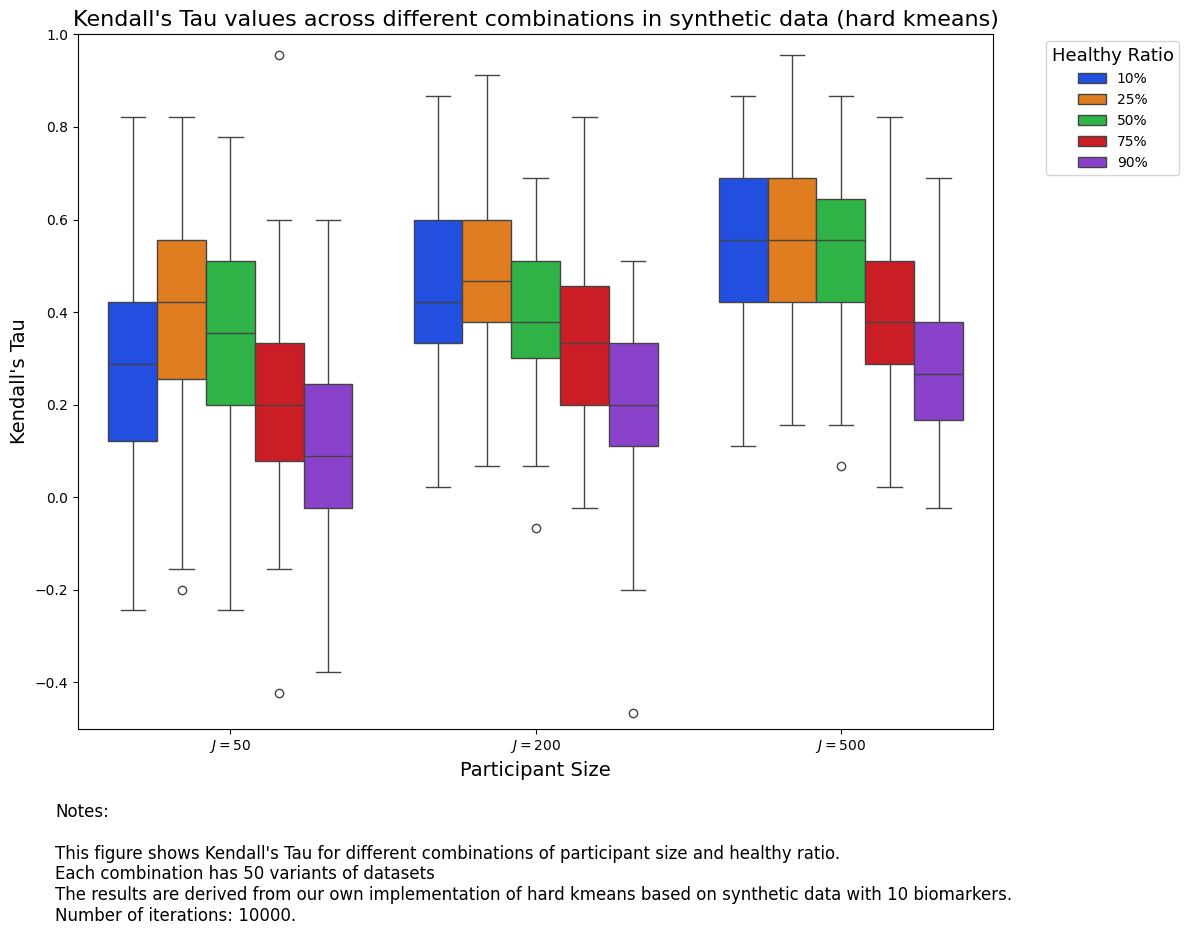
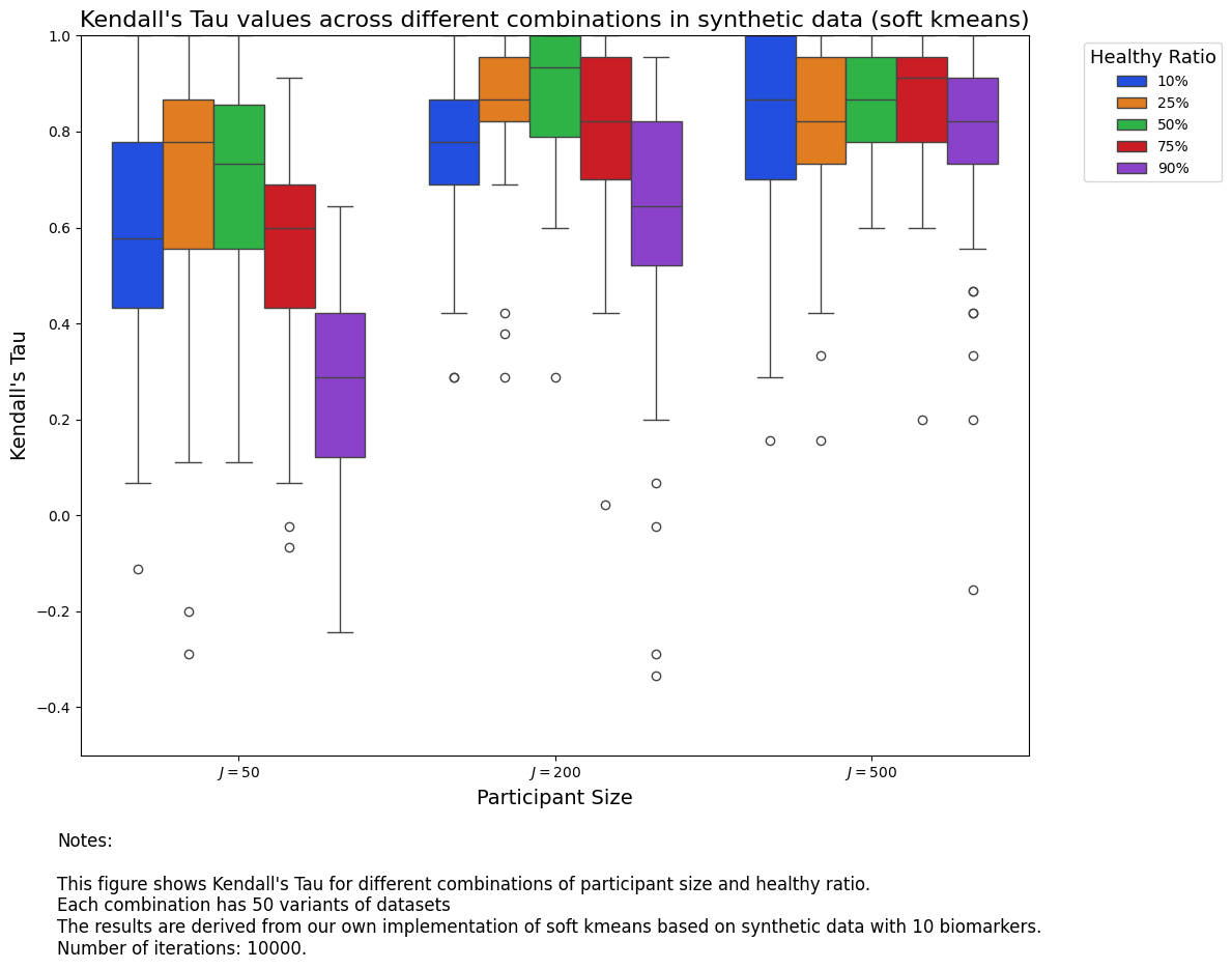
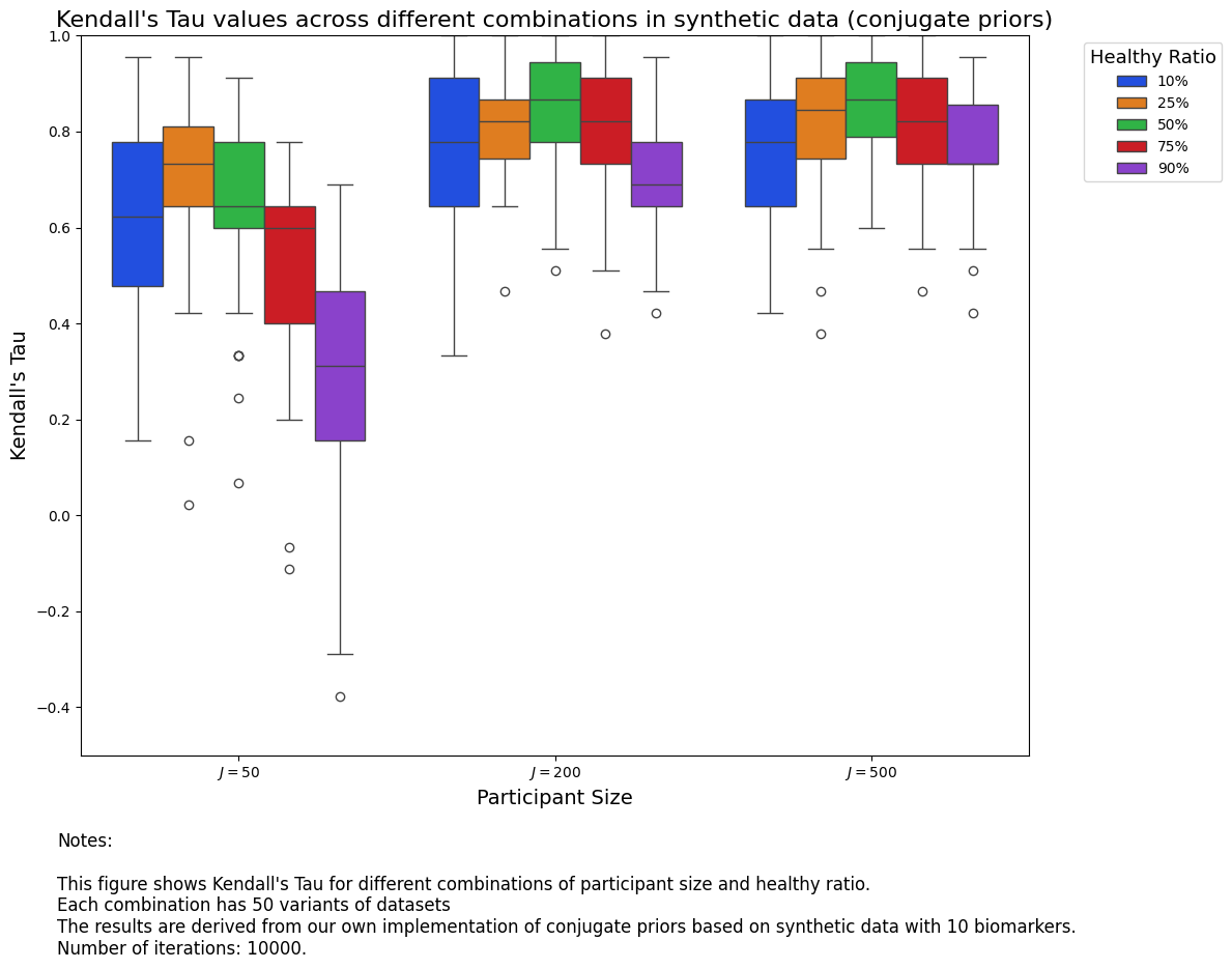
From the two results, we are able to see that it is better to have more participants, because that offers more information for our models. In terms of healthy ratio, it seems \(50\%\) is a sweet spot.

Also, we notice that conjugate priors perform better than soft K-Means.

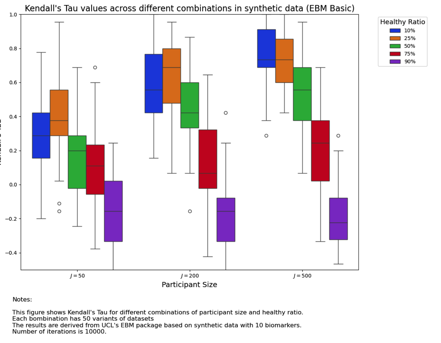
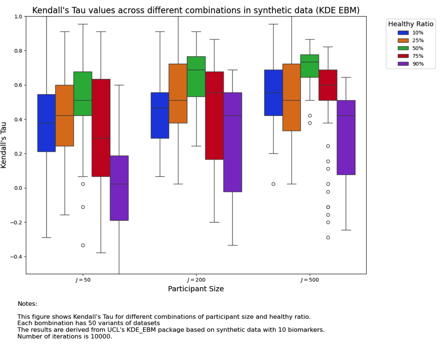
We also tested the two algorithms developed by UCL POND group with the same 750 datasets: EBM Basic and KDE EBM. See the following for results:

Figure 10.4: Results of EBM

The parameters we used in the package of ebm are:

• n_iter = 10000
• greedy_n_iter=10
• greedy_n_init=5

More specific configurations can be found at https://github.com/hongtaoh/ucl_ebm/blob/master/implement/calc_tau_basic.ipynb

Figure 10.5: Results of KDE EBM

The parameters we used in the package of kde-ebm are:

• n_iter = 10000
• greedy_n_iter=10
• greedy_n_init=5

More specific configurations can be found at https://github.com/hongtaoh/ucl_kde_ebm/blob/master/implement/calc_tau_basic.ipynb

We can see that the performance of KDE EBM is more stable but EBM basic performs well when the healthy ratio is below \(50\%\).

Neither of these methods had results as good as conjugate priors. We have to point out that, even though their accuracy is not as high, their speed is really high. Both of these two algorithms can generate results with a single laptop GPU in just one hour; however, it might take days for our algorithms.